

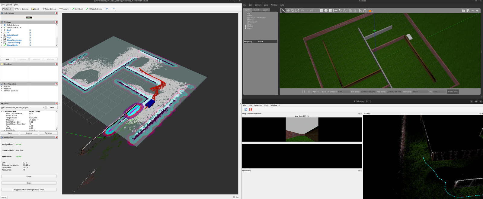
I wanted a robot I could develop perception and navigation on without waiting for hardware, and I wanted to find out whether a robot could get by on stereo cameras alone. Most indoor mobile robots lean on a lidar. A lidar gives you clean range measurements and forgives a great deal. Take it away and every mistake in the camera model shows up immediately as a broken map.
So I built the robot twice. Once as a simulated machine in Gazebo, with a physics model and noise-bearing sensors, and once as a physical stereo camera on my desk with its own driver. Both feed the same SLAM and navigation stack. This is a write-up of how it works and, more usefully, of what fell out of comparing the two.
The simulated robot
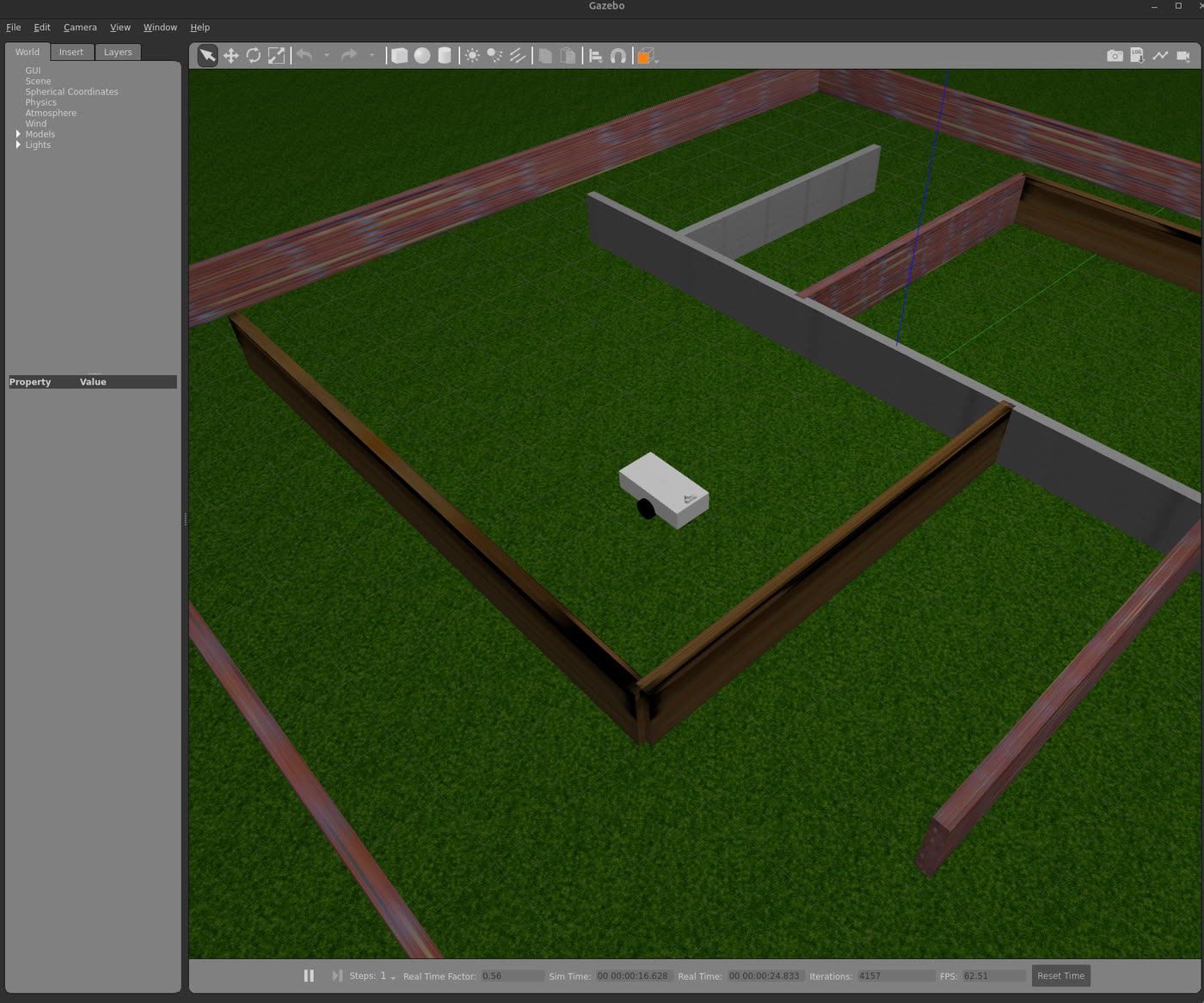
The robot is a differential-drive platform in a 20 by 20 metre maze. The interesting part is the physics settings rather than the geometry, because those decide whether what you see in the simulator means anything.
Physics runs on ODE with a 4 millisecond step and 10 solver iterations. Contact is parameterised per surface: friction 1.5 at the drive wheels against 0.01 at the casters, with contact stiffness and damping set so the chassis neither sinks into the floor nor slides across it. Every link carries a real mass and a full inertia tensor, 50 kg for the base and 5 kg per wheel, rather than the placeholder values a model tends to accumulate.
The sensors carry noise, which matters more than it sounds. It is easy to build a simulated camera that returns a perfect image and a simulated IMU that returns the exact truth, and then to discover that your filter was quietly relying on that. Gaussian noise sits on all six IMU axes at 100 Hz, on both camera images, and on GPS position and velocity.
Seeing without a lidar
The perception chain starts with a 120 mm stereo baseline. That figure is declared once in the robot description and drives both where the camera links sit and what the camera plugin reports as its projection, so the geometry and the optics cannot drift apart as the model is edited.
From there: rectification, disparity, and a point cloud. RTAB-Map takes the stereo pair and builds the map, closing loops when it recognises somewhere it has been.
The navigation stack still wants a 2-D scan for its obstacle layer, and there is no lidar to provide one. So the scan is synthesised from the stereo point cloud, keeping returns between 0.25 and 1.5 metres above the base. The lower bound is what stops the floor being read as a wall. It is a small piece of plumbing that decides whether the robot can move at all.
Navigation, and getting unstuck
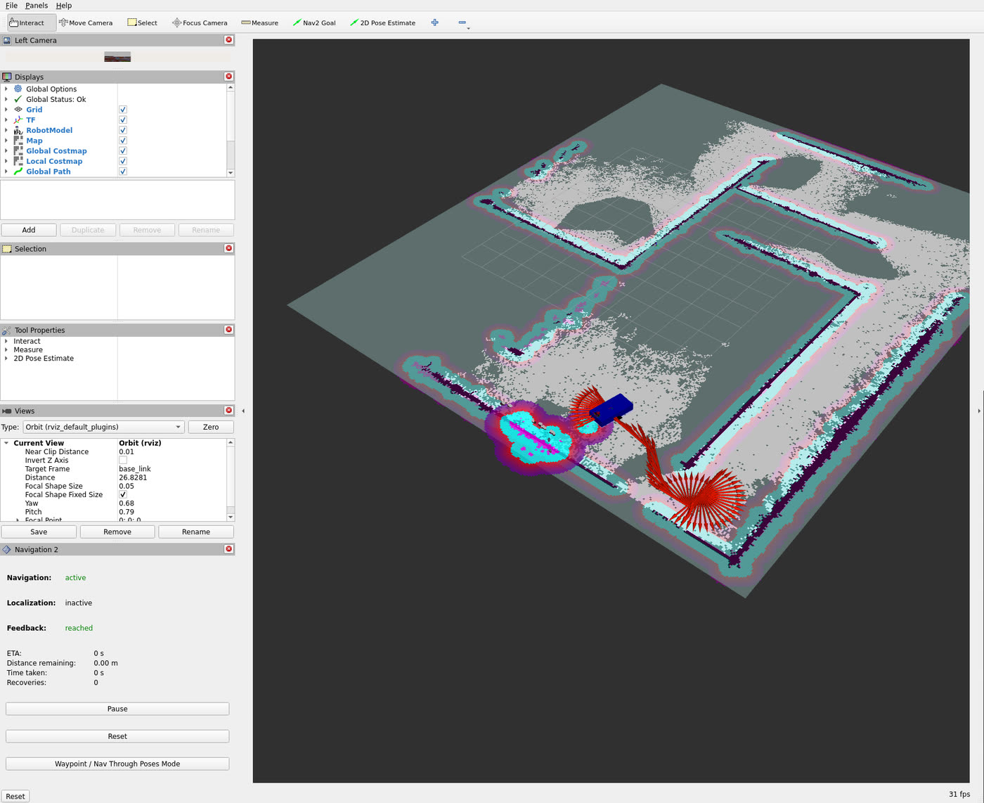
Navigation is Nav2, with the full lifecycle: planner, controller, smoother, behaviour server, waypoint follower and velocity smoother. Bringing all of that up alongside Gazebo, the stereo pipeline and RTAB-Map means roughly 37 nodes starting in a staged order.
I wrote custom behaviour trees rather than taking the stock one. A robot in a tight maze corridor spends a surprising amount of its life wedged against a wall it cannot see well, and the default recovery set gives up too early. The tree clears the local costmap, then the global one, then spins, backs up half a metre, spins the other way, and waits. It will do that a great many times before declaring failure. That is stubbornness rather than elegance, and in a maze stubbornness is what gets you to the goal.
Testing it like software, not like a demo
A simulation you watch is a demo. A simulation that can fail a build is a test. The difference is whether anything asserts.
So a scenario here is a start pose, a goal pose and a time budget, and the harness asserts two things: clearance never drops below 0.15 m, and the robot finishes within 0.5 m of the goal before the timeout. It runs headless with no display and exits 0 or 1, which is all a CI job needs.
It also records the numbers you would want to regress on rather than just pass or fail: the minimum clearance actually reached, the distance actually driven, and the time to goal. A run can pass while quietly getting worse, and that only shows up if you keep the measurements. Failures are separated by cause (collision, planner failure, timeout) because those three want different responses.
The most useful thing the harness told me was not a failure. It was a passing run whose recovery count had climbed from 10 to 58.
The same camera on the bench
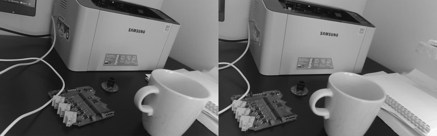
The hardware half is an ELP global-shutter stereo module. It presents itself as one USB camera delivering a single 2560 by 800 side-by-side frame at up to 120 fps, which is not something ROS can consume directly.
So the driver is mine: about a thousand lines across three nodes. A splitter cuts the side-by-side frame into left and right streams with matching camera info, rectifies from the calibration files and uses threaded capture to hold the frame rate. A CUDA node runs stereo matching on the GPU and falls back to CPU when there is no CUDA device. A third node pairs semi-global block matching with WLS filtering for the cases where disparity quality matters more than latency.
The calibration cross-checks, which is the part worth verifying rather than trusting. The right camera projection matrix carries a translation term of −40.058 against a focal length of 669.515. Divide one by the other and you get a 59.8 mm baseline, against the 60 mm the hardware is built to. In simulation the disparity message reports 0.120 m, matching the 120 mm in the robot description. Both halves agree with themselves.
Depth, and two ways to get it wrong
Computing disparity from that pair produced two mistakes worth recording, because both look fine until you check.
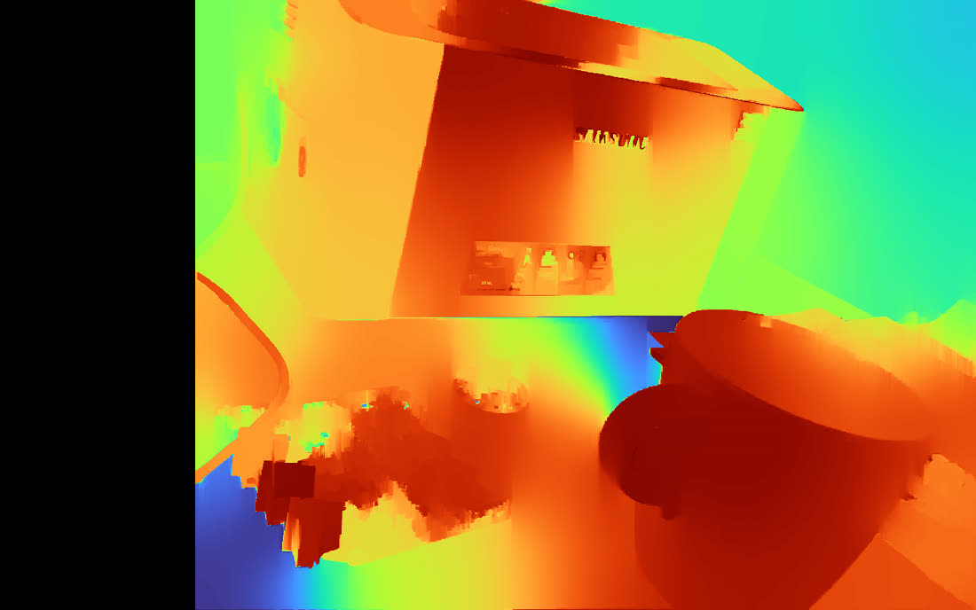
The camera is mounted inverted, so the frames need rotating. Rotate a stereo pair by 180 degrees and the eyes have to swap as well, because the horizontal order reverses. Rotating without swapping still yields a disparity map that looks plausible at a glance. It resolved 44.5% of pixels instead of 87.2%, and gave a depth field that was quietly wrong.
Then the first corrected map reported a higher valid-pixel count than the one I ended up keeping. It was saturating: with a 128-pixel search range, 25% of pixels were pinned at the limit because the scene was closer than the range could represent. Widening the search to 256 pixels dropped the headline number from 90% to 80% and made the depths correct. The worse-looking metric was the honest one, which is a good thing to be reminded of before you start reporting metrics to anybody else.
SLAM on the hardware
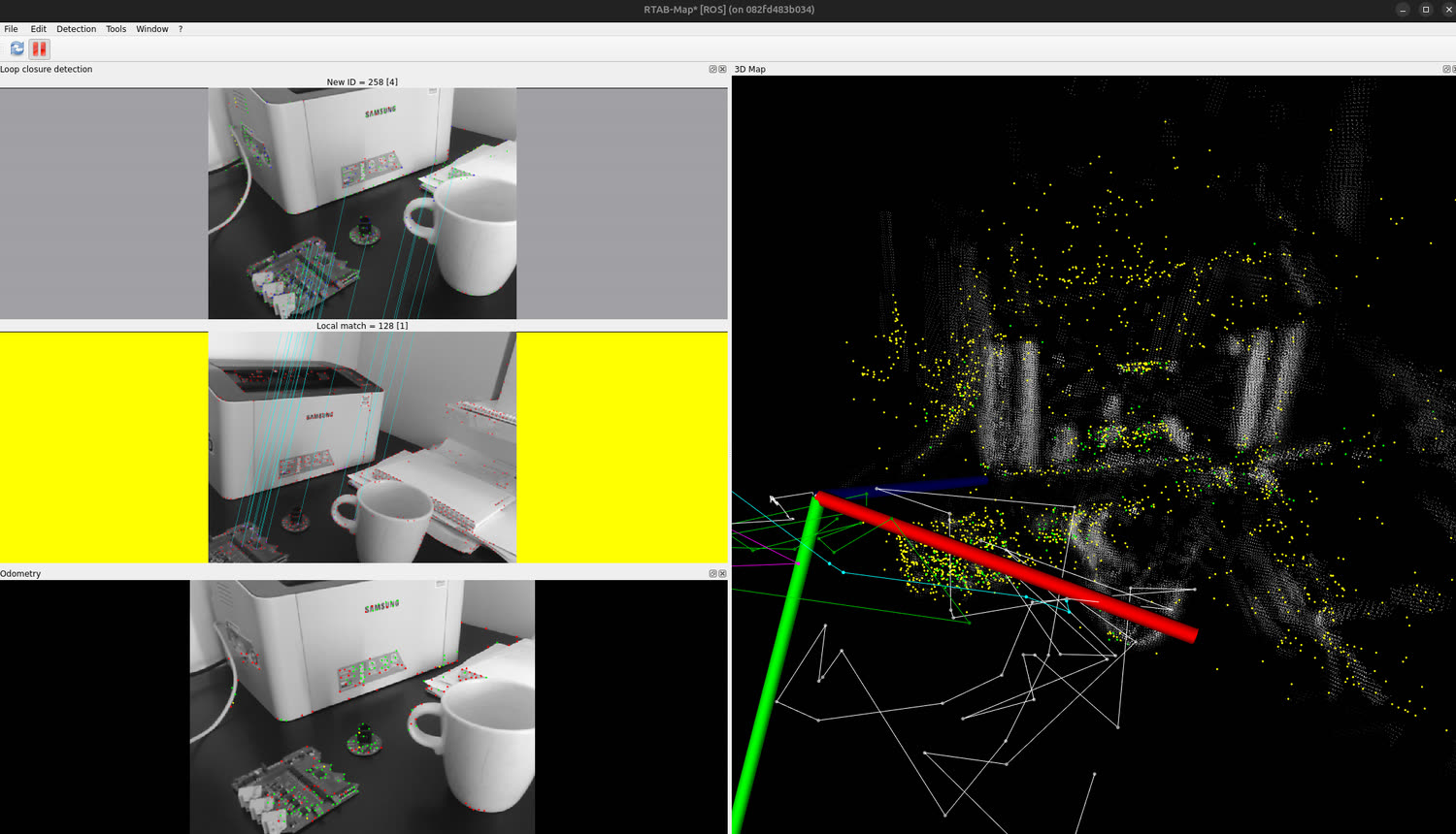
With the driver working, the physical camera runs the same RTAB-Map configuration as the simulated robot. Carrying it around the desk, visual odometry tracks on 150 to 190 inliers and the map fills in.
The screenshot below is the moment the thing earns its keep: node 258, and a local match of 128 feature correspondences against an earlier view of the same desk. The cyan lines are the correspondences. That is the system recognising it has been here before, on real images, with no lidar involved.
Cameras give you more than geometry
Choosing cameras over a lidar costs you clean range data. What you get back is an image, and an image can answer questions a range sensor cannot.
Right now the stereo pair is used purely for geometry: disparity, a cloud, a map. The same rectified frames are already on the ROS graph, so a learned perception node is additive rather than a rebuild. Subscribe to the topics that exist, publish something new alongside them. That is the practical argument for a camera-first robot, and it is why the pipeline is worth getting right before anything clever goes on top.
The obvious next node is detection and segmentation, because geometry alone cannot tell you what it has found. An occupancy grid says a cell is occupied. It does not say the obstacle is a cable, a sock, a chair leg or a pet, and those want different behaviour: drive around one, refuse to touch another, treat a third as something that will have moved by tomorrow. Feeding a semantic layer into the costmap changes the robot from avoiding shapes to avoiding things.
The compute is already in place for it. The container builds OpenCV and RTAB-Map from source with CUDA, and running inference beside the SLAM stack on the same GPU is a scheduling problem rather than a new architecture. TensorRT covers the deployment side when a model needs to hold a frame rate on constrained hardware.
Simulation helps here in a way that is easy to miss. Training data has to be labelled, and labelling is the slow, expensive part. A simulator knows exactly what every object is and where it sits, so it can emit perfectly labelled frames as fast as it can render them, including for the awkward cases you would struggle to stage safely in a real room. The same virtual environment that tests navigation can generate the training set for the perception that navigation depends on.
Getting it off the desk
The honest gap in all of this is that the chassis is simulated and the camera sits on a desk. The next piece of work is the machine underneath, and that is electronics rather than software.
The plan is a small differential-drive platform built around a board I design: motor drivers with current sensing, quadrature encoder inputs, an IMU, power management and a battery stage, with an STM32 running the real-time loop and talking to ROS 2 over USB or Ethernet. Nothing exotic. The reason to design it rather than assemble it from modules is that the timing-critical parts want to be deterministic and close together. Encoder counting, current limiting and the motor commutation loop belong in firmware on one board with a known layout, not spread across three dev boards connected by jumper wires whose behaviour changes when you nudge them.
That split matters for what sits above it. If the base board guarantees the wheel odometry and the safety cut-out, then ROS 2 is free to be late occasionally without the robot doing something stupid. Drawing the line between hard real-time firmware and soft real-time middleware is one of the decisions that is expensive to change later, so it is worth making deliberately at the start.
The point of building it is to close the loop. The test harness already drives scenarios against the simulated robot and asserts on clearance and goal tolerance. Pointing that same harness at a physical machine, and watching where the numbers diverge, is the only way to find out how much the simulation has been telling the truth.
What comparing the two actually taught me
This is the part I did not expect, and it is the reason building both halves was worth the time.
The real desk scene resolved 80% of its pixels. The simulated maze, on its flat walls, rejected most of its stereo correspondences and produced almost nothing. RTAB-Map was logging 377 of 388 correspondences rejected on some frames. The simulation was harder than reality for the perception stack, not easier.
That inverts the usual worry. The familiar failure is a simulation that flatters your algorithm, so everything works in the virtual world and falls over on the robot. Here the opposite was true. A stereo matcher tuned until it passed in that maze would have been tuned against a problem the robot never actually faces. Either way the conclusion is the same: a simulation is not automatically a fair test, and the only way to find out which way it is unfair is to build the physical half and compare.
The second lesson was about timing. The robot description asks the cameras for 30 Hz. Under load they do not deliver it. If perception is being tested at a few hertz in simulation but runs at thirty on the robot, the test is not representative, and that gap belongs in the test report rather than in a footnote.
Where this leaves the platform
What exists now is a robot that maps and navigates from two cameras in simulation, the same perception chain running on a physical stereo camera, and a test harness that can drive scenarios headless and fail on a number rather than an opinion.
The next step is the one I have not done yet: putting the scenario suite into a pipeline so it runs on every change, with the metrics tracked across builds instead of noted down as they go past. The pieces are there, since the stack is containerised and the tests run without a display and return an exit code, but the pipeline itself is still a shell script I run by hand.
After that it is the base board and the perception nodes, in that order. Hardware first, because a real chassis is what turns the test harness from a simulation exercise into a measurement of something physical.